In this section, you will be able to describe the complexity of an algorithm via Big O notation. You will learn how to trace and analyse time complexity in three searching and two sorting algorithms.
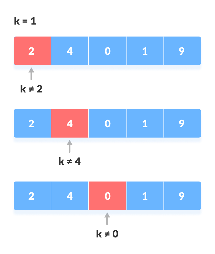
From GCSE, you will know that a linear search is where you go along a list and check every item to see if it matches what you want. You will also know that a linear search is effective on short lists, but extremely ineffective on longer ones.

At A Level, we aren't that general. You may know that linear functions are graphs with a straight line. Linear search's efficiency is inversely proportional (if you don't know what that is, retake GCSE Maths) to the number of items in it, which we call n. We therefore give it the time complexity O(n).
The equation for a straight line is y = ax + c. And as x increases, the constant has proportionally less effect on the value of the function.
This is what we call Big O notation. It was invented by German number theorist George Landau.
The idea with time complexity is to design alorithms which run quickly whilst taking up minimal resources such as memory. To compare the execution time, we compare the number of operations or steps the algorithms need, in terms of the number of items to be processed.
When complexity is evaluated, not all parts are equal. Take, for example, the equation 4 + 3n + 1. Only the 3n has any real significance, as it is the only part of the equation with any impact.
A mathematical function maps one set of values to another. Take the set {1, 2, 3}, to be mapped to the set {2, 4, 6}. The function we have for this is f(x) = 2x. In this set, every element of the domain (the input values), is related to exactly one element of the co-domain (the output values).
We have different time complexities with diffent Big O Notation results for each.
Constant complexity is the crème-de-la-crème of time complexity, and everyone wants to be like it. It is constant, so it takes the same time to complete the task however many items it has to do it for. A good example is finding the first item in a list. Its Big O notation is O(1).
Logarithmic complexity is the next-best thing. The time complexity decreases as the number of items increases. A good example is a binary search, or a binary tree search (see 4.2.5). Its Big O notation is O(log(n)) (logarithms are the inverse of powers; look it up).
Linear complexity comes next. Its time complexity is O(n).
Polynomial complexity is afterwards. A polynomial is an equation with a variable, constant and exponent. A good example is a bubble sort. Its Big O notation is O(n²).
Exponential complexity is after that. An exponential is where an equation takes the power, instead of the base. A good example is an intractable problem (more on them later). Its Big O notation is O(2^n) (compare to polynomial).
Factorial complexity is the least efficient. A factorial is a number multiplied by all the numbers before it. A factorial is represented by an exclamation mark (i.e. 3! = 3 × 2 × 1 = 6). A good example is brute forcing an algorithm. Its Big O notation is O(n!).
It might be useful to know that a merge sort also takes logarithmic complexity, but its Big O notation is slightly different as O(n * log(n)).
In an exam you may be given a piece of code and asked to work out the time complexity. Here are a few general tricks:
A nested loop (a loop inside of another) is a polynomial, with time complexity O(n²). If the nested loop is in another nested loop, it has the complexity O(n³). On³ is used in 3D coordinates.